Lecture 21: Sorting Algorithms
- Selection Sort.
- Insertion Sort.
- Bubble Sort.
- Merge Sort.
Sorting
In the last lecture we compared two searching techniques: Linear Search and Binary Search. Binary Search relied on it's input array already being sorted. But how do we get that array sorted in the first place? Today we'll introduce 3 basic algorithms for sorting an array of elements: Selection Sort, Insertion Sort, and Bubble Sort.
In the implementation of each algorithm below it is only sorting an array of integers. Any other primitive type or object that can be compared could be used just as well. Remember that for objects we would have our objects implement the Comparable interface and define the compareTo method.
Last thing: the entries that we're sorting could also be thought of as keys representing lots of other data. The numbers I'm sorting could be random numbers given to customers waiting to be seated at a restaurant. Those with smaller "keys" would be seated first. However, just sorting those keys isn't helpful by itself. Along with the key values I would also need to update the satellite date that goes along with it: the customer's names. Using this "key and satellite data" method we can use these same sorting algorithms on almost anything.
Selection Sort
How Does Selection Sort Work?
First, here's some example code for Selection Sort. It starts by looking for the smallest element in the array. For sorting in increasing order, this element should be in position "0" in the array. What if the smallest entry is in poition "i" in the array? The algorithm swaps the value in position i with the value in position 0. This is done by using an extra variable to help with the swap.
	int temp = array[0];
	array[0] = array[i];
	array[i] = temp;
Swapping values like this is actually quite common - especially when sorting. What does our algorithm do after this first swap? It finds the second smallest entry in the array and swaps it into position 1. Then it finds the third smallest and swaps, then the fourth smallest and swaps, then the...
Correctness of Selection Sort
In a given iteration i of the algorithm, the value that should be placed in the position array[i] is found and swapped into that position. The swap is done with some array position with an index greater than i. Why? The array positions array[0 .. i-1] are already in their correct positions. So, we don't want to mess them up. Furthermore, since those are already in their correct positions, none of them will be the value that correctly goes into position array[i]. So, after looping through n iterations for an array with n elemetns, we get a correctly sorted array.
Running Time of Selection Sort
In the first iteration of the algorithm's loop we have to check all of the elements in an n-element array to find the smallest one. However, on the next iteration we can skip the first array entry since we know it won't count as the second smallest entry in the array (because it's already been found to be the smallest). So, that time we only have to check n-1 array entries.
On the next iteration of the loop we can now skip the first 2 entries, and only check n-2 entries. Then we only check n-3 entries, then n-4, etc. At the very end we only have one array entry left to check. So how long does all of this take? Well, the total number of array entries we checked was:
n-1 + n-2 + ... + 1
This is something called an arithmetic series. We can solve it by performing this neat little trick of making a copy of each value, then adding the copies to the originals (in the reverse order).
    (n-1 + n-2 + ... + 1 ) +
    ( 1  +  2 + ... + n-1)
  = n  +  n + ... +  n
This is just the value n added up n-1 times. Also, since we doubled the entries in the series, we'll have to divide by 2. Thus, our total value for the arithemtic series is n(n-1)/2. What does this mean for our running time? Well, the division by 2 is a constant factor, so we can ignore it. Now what about the subtraction of "1" ? Ignore it! This leaves us with a simple function for describing the running time: O(n2).
Insertion Sort
How Does Insertion Sort Work?
First up is a simple implementation of the Insertion Sort algorithm. From that code and from the applet above we can start inferring that the algorithm works a lot like most people would sort a hand of playing cards. We start with a section of card we have sorted, then we add or "insert" one more card into its proper place in that sorted section. Now we have a slightly larger sorted section. Eventually, after all of the cards are inserted into their place one after another, we'll have the entire hand of cards sorted.
Correctness of Insertion Sort
We start each iteration of the algorithm's loop with a subsection of the array already sorted. (When the algorithm first starts the first element by itself is our "sorted" subsection.) We then take the first array entry outside of this sorted subsection and swap it down the line. This continues until it reaches a point where the element before it is less than or equal to it and the element after it is larger (or maybe we just never swapped the element out of its old spot, in which case we don't yet know what comes after it). With this element inserted we've now increased our sorted subsection's size by 1. After n such iterations for an array with n elements we'll have the entire array sorted.
One thing to note about this algorithm is that we used a loop invariant. To show it's correctness. I've mentioned loop invariants before, but this is a particularly good example. In this case our loop invariant is that a subsection of the array, array[0 .. i], is sorted. At the start of each iteration is true. Then we increase i by 1 as we start to add one more element to the sorted order.
This messes up the loop invariant since the element in entry array[i] may now be smaller than some of the elements before it. However, our algorithm swaps this element down the line as far as it need to go in order to correct this problem. Thus, the loop invariant was true before and after each iteration of the loop.
Running Time of Insertion Sort
When we analyzed Selection Sort things were pretty easy because the algorithm did the same thing regardless of the initial array that it was given. With Insertion Sort things are a bit more tricky. We'll only swap the next element to insert as many times as we have to swap it. If its smaller than all of the elements already in the sorted subsection this takes a lot of swaps. If its larger than all of those elements we don't have to make any swaps. How do we account for this.
The case where the element being inserted is the new smallest element causes the worst case behavior of our Insertion Sort algorithm. This causes us to make a swap for every element already in our sorted subsection. Again that means we get the arithmetic series:
1 + ... + n-2 + n-1 = n(n+1)/2
This is the same series that we had for Selection Sort, but now we get the values in reverse. The resulting runnning time is the same, though: O(n2) in the worst case.
Now what about the case where the element is larger than all of the elements in the sorted subsection? We don't have to make any swaps. So, if each iteration of the loop is like this we only do a constant amount of work each loop. That means only the number of loops is important (because we always drop constant factors). Thus, this is the best case behavior for the algorithm and gives a running time of only O(n). How could this happen? If the array was already sorted when it was given to us.
Between the extremes of worst case and best case is the average case behavior of the algorithm. This is what we would normally expect from it (such as the case of getting randomly arranged input). For Insertion Sort, we could use probability theory to find that on average we could expect each new element to be inserted into about the middle of the old sorted subsection. This would mean the average case requires about half the number of swaps that the worst case required. Does this matter asymptotically? Nope. The asymptotic running time is still the same as in the worst case: O(n2).
Bubble Sort
How Does Bubble Sort Work?
First up, a simple coding implementation of Bubble Sort. Bubble Sort is an odd algorithm, not one you would use in practice, but one I should probably mention so that you know what it is. It works almost like a cross between Selection Sort and Insertion Sort. We start at the top of the array and keep a sliding window of two array entries: array[i] and array[i-1]. Since we're sorting in ascending order, if the value in entry array[i] is less than the value in entry array[i-1], we swap the two entries. We then decrease i by one and repeat the comparison. After we've reached the bottom, i=1, we restart at the top of the array. This continues for n loop iterations for an array with n elements.
The sliding window idea can be a bit tricky, so here's another thought: think of this as working like Selection Sort. We're really just starting at the top of the array and remembering the smallest element we've found so far. We then keep swapping this element down the line until we find a new smallest element (and switch to that new element) or the element we're moving has been added to the sorted order. Just like with Selection Sort we don't have to keep checking once we've reached the sorted subsection of our array. We already know that subsection is solved, so we can skip it and start on the next iteration of the loop sooner.
Correctness of Bubble Sort
Bubble Sort's proof of correctness is the same as for Selection Sort. It first finds the smallest element and swaps it down into array entry 0. Then finds the second smallest element and swaps it down to array entry 1, then the third, fourth, etc. It never messes with the previously sorted subsection of the array so it never undoes previous work. After n iterations through this loop on an array with n elements we have a totally sorted array.
Running Time of Bubble Sort
It's running time is also just like Selection Sort. We have to start at the top of the array each iteration and move down comparing (and maybe swapping) until we reach the previously sorted subsection of the array. Each iteration increases or sorted subsection size by 1, so we perform one fewer comparison each loop iteration. This gives the same arithmetic series and total result:
n-1 + n-2 + ... + 1 = n(n+1)/2
The best case, worst case, and average case running times are all the same asymptotically: O(n2).
Reviewing Selection, Insertion, and Bubble Sort
In the last lecture we covered 3 different sorting algorithms. Here's a quick review of those 3 before we move to a couple more complicated algorithms.
- Selection Sort
- Algorithm: Find the next smallest element and add it to the end of our growing sorted subsection.
- Analysis: Same O(n2) running time regardless of input. So, can say that it has a &Theta(n2) running time.
- Insertion Sort
- Algorithm: Insert the next given element into the proper place in the already sorted subsection.
- Analysis: Runs in O(n) time in the best case - when it's given an array that's already sorted. However, it's worst case running time is still O(n2). It's average case running time is also O(n2). Because it's running time varies between these extremes, we can not state any &Theta bound about it.
- Bubble Sort
- Algorithm: Starting with the rightmost pair of array entries keep moving left and swap entries whenever the left entry is larger than the right entry. Repeat n times for an array with n entries.
- Analysis: Same running time regarless of input: O(n2). So, we can also say that Bubble Sort runs in &Theta(n2) time to give a tight bound. (Yes, if given a pre-sorted array Bubble Sort will make fewer swaps - but it will still have to check all of those entries. Thus, still a O(n2) running time.)
Merge Sort
In most cases all of our previous sorting algorithms ran in O(n2) time. Now we've finally got an algorithm that beats that bound and gives a O(n lg n) running time. Asymptotically this is a tremendous improvement over our previous sorting algorithms. Just remember the comparison we had about the growth of n versus lg n when we looked at Linear Search vs. Binary Search. For large cases we'll get the same kind of tremendous improvement by using Merge Sort instead of one of our 3 previous algorithms. However, there are two minor problems with Merge Sort.
- Remember that the O-notation for running times ignores constant factors. The constant factors for Merge Sort are larger than for the 3 previous algorithms. Still, for large problem sizes these constant factors won't matter.
- All of our previous algorithms sorted "in place". That means they only needed one array to handle everything (plus a single holder variable for swapping array entries). For Merge Sort a single holder variable won't work. We need an entire second array to have enough workspace. If the space requirements for our program were really tight this might be a problem. Usually, though, if we have enough space for 1 array we probably have enough room for 2.
Divide and Conquer
How does Merge Sort get its running time down to O(n lg n)? By using a common computer science tactic: divide and conquer. In computer science this means that we divide up a given problem into two smaller, easier problems. We then recursively solve these two smaller problems. Once both of those are solved, we then combine those mini-solutions together to solve our original problem. Here's a cleaner description:
- Divide: If the problem is small enough, just solve it. Otherwise divide it into two or more smaller problems and recursively solve those.
- Combine (Conquer): Once the smaller sub-problems are solved, combine them to solve the original problem.
This works much like our recursive fractal designs. The difference is that now we are calculating something (a sorted array) and we must combine the values returned by our recursive calls. How does this work in Merge Sort? In this code Merge.java we've got a recursive method mergeSort that sorts an array. Here's how the divide-and-conquer method works.
- Divide: If the problem is small enough, just solve it. Otherwise make 2 recursive calls to
mergeSort: one on the top half of the array and one on the bottom half of the array.
- Combine (Conquer): We we made recursive calls and those returned we've now got each half of the array sorted individually. Now we need to get the entire thing sorted. We do this by combining the the two sorted subarrays in linear time (O(n)-time).
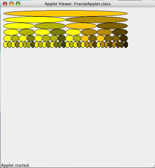
We'll get to the "merging" part in just a moment. First stop to make sure you understand how the "divide" part is operating. We start out with an array of n elements. We'll first try to recursively solve the top and bottom halves seperately. Each of those will have n/2 elements. Consider just one of those recursive calls, say, the top half. Those n/2 elements are still probably too much. So, we'll recursively solve each half of that portion of the array: n/4 elements in each of those sections. These recursive calls continue down until we get to a small enough sub-problem that we'll finally just solve it. If we keep going until the problem size is just a single element? Well, it takes lg(n) such divisions to get from n down to 1, so we'll have lg(n) recursive stages. At each stage there will be O(n) work total whenever we have to "merge" things together. Remember the "eggs" portion of our current homework? The picture it draws is actually very similar to what we're doing here in recursively dividing our array.
Linear Time Merging
We've now seen how merge sort keeps making recursive calls to put off doing any actual sorting. So what if we've finally got two recursive calls that return? How can we possibly merge those two sorted subsections together in linear time? Well, we'll be using the fact that those subsections are individually sorted and that we've got a second empty array where we can store things. Let's assume that the table below shows two sorted sections that we want to merge. How would we go about doing that?
| Section 1 | Section 2 | Spare |
| 1 | 3 | |
| 5 | 4 | |
| 6 | 12 | |
| 19 | 14 | |
| 21 | . | |
| . | . | |
| . | . | |
| . | . | |
| . | . | |
| Section 1 | Section 2 | Spare |
| . | 3 | 1 |
| 5 | 4 | |
| 6 | 12 | |
| 19 | 14 | |
| 21 | . | |
| . | . | |
| . | . | |
| . | . | |
| . | . | |
| Section 1 | Section 2 | Spare |
| . | . | 1 |
| 5 | 4 | 3 |
| 6 | 12 | |
| 19 | 14 | |
| 21 | . | |
| . | . | |
| . | . | |
| . | . | |
| . | . | |
| Section 1 | Section 2 | Spare |
| . | . | 1 |
| 5 | . | 3 |
| 6 | 12 | 4 |
| 19 | 14 | |
| 21 | . | |
| . | . | |
| . | . | |
| . | . | |
| . | . | |
| Section 1 | Section 2 | Spare |
| . | . | 1 |
| . | . | 3 |
| 6 | 12 | 4 |
| 19 | 14 | 5 |
| 21 | . | |
| . | . | |
| . | . | |
| . | . | |
| . | . | |
| Section 1 | Section 2 | Spare |
| . | . | 1 |
| . | . | 3 |
| . | 12 | 4 |
| 19 | 14 | 5 |
| 21 | . | 6 |
| . | . | |
| . | . | |
| . | . | |
| . | . | |
| Section 1 | Section 2 | Spare |
| . | . | 1 |
| . | . | 3 |
| . | . | 4 |
| 19 | 14 | 5 |
| 21 | . | 6 |
| . | . | 12 |
| . | . | |
| . | . | |
| . | . | |
| Section 1 | Section 2 | Spare |
| . | . | 1 |
| . | . | 3 |
| . | . | 4 |
| 19 | . | 5 |
| 21 | . | 6 |
| . | . | 12 |
| . | . | 14 |
| . | . | |
| . | . | |
| Section 1 | Section 2 | Spare |
| . | . | 1 |
| . | . | 3 |
| . | . | 4 |
| . | . | 5 |
| . | . | 6 |
| . | . | 12 |
| . | . | 14 |
| . | . | 19 |
| . | . | 21 |
Merge Sort In Action