When you submit your work, follow the instructions on the submission workflow page scrupulously for full credit.
Instead of handing out sample exams in preparation for the midterm and final, homework assignments include several problems that are marked marked Exam Style . These are problems whose format and contents are similar to those in the exams, and are graded like the other problems. Please use these problems as examples of what may come up in an exam.
As a further exercise in preparation for exams, you may want to think of other plausible problems with a similar style. If you collect these problems in a separate notebook as the course progresses, you will have a useful sample you can use to rehearse for the exams.
Is this assignment properly formatted in the PDF submission, and did you tell Gradescope accurately where each answer is?
This question requires no explicit answer from you, and no space is provided for an answer in the template file.
However, the rubric entry for this problem in Gradescope will be used to decuct points for poor formatting of the assignment (PDF is not readable, code or text is clipped, math is not typeset, ...) and for incorrect indications in Gradescope for the location of each answer.
Sorry we have to do this, but poor formatting and bad answer links in Gradescope make our grading much harder.
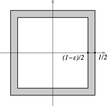
Let $d$ be a positive integer. Given a positive real number $a$, the set $$ C(d, a) = \{\mathbf{x}\in\mathbb{R}^d \ :\ -a/2 \leq x_i \leq a/2 \;\;\text{for}\;\; i=1,\ldots,d\} $$ is a cube of side-length $a$, centered at the origin. The unit cube is $C(d, 1)$.
Let $\epsilon$ be a small positive real number ($0<\epsilon \ll 1$). The $\epsilon$-skin $E(d, \epsilon)$ of the unit cube $C(d, 1)$ is a layer of thickness $\epsilon/2$ just inside the surface of $C(d, 1)$: $$ E(d, \epsilon) = C(d, 1) \setminus C(d, 1-\epsilon) $$
where the backslash denotes set difference.
The figure below shows the $\epsilon$ skin $E(2, \epsilon)$ in gray for some small $\epsilon$.
The volume of a compact set $\mathcal{A}\in\mathbb{R}^d$ is the integral of $1$ over $\mathcal{A}$.
What is the volume $c(d, a)$ of $C(d, a)$ and, in particular, what is $c(d, 1)$? No need to prove your answers.
Give a simple formula for the volume $e(d, \epsilon)$ of $E(d, \epsilon)$ in terms of $d$ and $\epsilon$.
Approximate the formula for $e(d, \epsilon)$ you gave for the previous problem to first order in $\epsilon$. That is, approximate $e(d, \epsilon)$ with an affine function of $\epsilon$. Explain very briefly how you derived the approximation.
If your approximation were exact, for what (approximate) dimension $d$ would the $\epsilon$-skin $E(d, \epsilon)$ take up all of the cube's volume? Give your answer as a function of $\epsilon$.
Of course, your approximation in the previous problem is not exact, or else it would not be an approximation. Also, the $\epsilon$-skin will never take up all of the cube's volume, just most of it. So now we do a more accurate calculation numerically. Specifically, use the function matplotlib.pyplot.loglog to plot $e(d, 10^{-3})$ for $d$ between $1$ and $10^{6}$ and with logarithmic scaling on both axes. Label the axes meaningfully.
Are the numerical results approximately consistent with your approximation?
Let $\mathbf{p}$, $\mathbf{q}$, $\mathbf{r}$ be three points on the plane. Assume that the three points are not aligned.
A Voronoi diagram of the three points above can be formed by dividing the plane into 3 regions using three half-lines with a common origin at $\mathbf{z}$. Give the equations of the three lines $\ell_{pq}$, $\ell_{qr}$, $\ell_{rp}$ that contain the half-lines, and also give an expression for the coordinates of $\mathbf{z}$.
Show your derivation succinctly. Each line equation has a similar derivation, so show the derivation for just one and the final formula for all three. See the notes below for more detail on the format of your answers.
Also answer the following questions:
Write Python code that takes three points $\mathbf{p}$, $\mathbf{q}$, $\mathbf{r}$ on the plane as the three rows of a $3\times 2$ numpy array points and draws both the points and the three half-lines of their Voronoi diagram.
Specifically, write a function with header
def voronoi_3(points):
that returns numpy arrays z and u. The 2D-vector z is the origin $\mathbf{z}$ of the Voronoi diagram, computed with your formula from the previous problem. The $3\times 2$ numpy array u has as its rows unit vectors that point along the directions that define the three half-lines of the Voronoi diagram of the three points.
Then write a function with header
def draw_voronoi_3(points, z, u):
that takes points as above and the outputs z, u from voronoi_3 and draws the three points and their Voronoi diagram (three half-lines).
Show your code and the result of running it on the three triples of points test_points[t] for t $=0, 1, 2$, where test_points is defined as follows:
import numpy as np

test_points = np.array(
    [
        [[2., 0.], [0., 3.], [-4., -1.]],
        [[0., 0.], [0., 2.], [3., 0.]],
        [[-4., -1.], [3., 3.], [0. ,0.]]
    ]
)
Follow the notes below for programming and picture format.
The point of this problem is to verify the calculations done in the previous problem, so you are obviously not allowed to use any existing code that computes Voronoi diagrams. Your code only needs to work for three points on the plane.
Feel free to define additional helper functions to structure your code cleanly.
where $\alpha$ is a nonnegative parameter and $\mathbf{u}$ is one of the three rows of the array u. To obtain $\mathbf{u}$ from $\mathbf{a}$, note that these two vectors are perpendicular to each other, since $\mathbf{a}$ is perpendicular to the line while $\mathbf{u}$ is along it. So if $\mathbf{a} = (a_x, a_y)$, then $\mathbf{u}$ is a normalized version of either $\mathbf{v} = (a_y, -a_x)$ or $-\mathbf{v} = (-a_y, a_x)$.
A slightly trickier issue is to figure out whether to use $\mathbf{v}$ or $-\mathbf{v}$, so that its normalized version $\mathbf{u}$ points along the correct half-line. The key idea is that the half-line that bisects, say, $\mathbf{p}$ and $\mathbf{q}$ must be closer to either of these two points than it is to $\mathbf{r}$. So you can first pick $\mathbf{v}$, check if the point $\mathbf{z} + \mathbf{v}$ (which is an arbitrary point on one of the two possible half-lines) is closer to $\mathbf{p}$ than to $\mathbf{r}$ and, if not, replace $\mathbf{v}$ with $-\mathbf{v}$. Then normalize the result to have unit norm.
Your plots should be in three subplots plt.subplot(1, 3, i) of a single figure.
Plot the three points in p as blue dots (make them visible by using a large enough marker, say ms=15). Then plot the three half-lines of the Voronoi diagram in black.
Draw a long enough segment of each half line so that the diagram makes visual sense.
Set the subplot axis aspect to 'equal' to ensure that a unit on the horizontal axis is equal in length to a unit on the vertical axis.
Check visually that your results make sense. If not, you have a mistake either in the formulas or in the code. Debug and repeat.
The function retrieve defined below and the subsequent code retrieve and load a dictionary ames with keys 'X' (capitalized) and 'y' (lowercase) that contain the data used to make the plots in Figure 4 of the class notes on nearest-neighbor predictors.
from urllib.request import urlretrieve
from os import path as osp
import pickle


def retrieve(file_name, semester='fall22', course='371', homework=2):
    if osp.exists(file_name):
        print('Using previously downloaded file {}'.format(file_name))
    else:
        fmt = 'https://www2.cs.duke.edu/courses/{}/compsci{}/homework/{}/{}'
        url = fmt.format(semester, course, homework, file_name)
        urlretrieve(url, file_name)
        print('Downloaded file {}'.format(file_name))
file_name = 'ames.pickle'
retrieve(file_name)
with open(file_name, 'rb') as file:
    ames = pickle.load(file)
Using previously downloaded file ames.pickle
The numpy array ames['X'] is a $1379\times 1$ array with the home areas in square feet. The numpy array ames['y'] is a vector with $1379$ entries that represent the home prices in thousands of dollars.
The capital X stresses that this is a 2d array, while the lowerase y stresses that this is a 1d vector.
Use the class sklearn.neighbors.NearestNeighbors and its attribute function kneighbors to reproduce the plot in Figure 4 (b) of the class notes. The summary function used for $k$-nearest-neighbor regression when $k>1$ is the mean (it is OK to use numpy.mean).
Show your code and the resulting plot. No need to display the data points, just the three curves for different values of $k$. It's OK if the curve colors, figure aspect ratio, or placement of the legend are different. The plot is done with square footage varying from 0 to 6000 in increments of one (so there are 6001 points on each curve).
Important: You will get no credit if you use the class sklearn.neighbors.KNeighborsRegressor. This restriction is meant to drive home the point that most of the work for nearest-neighbor classification occurs in the data space $X$, and labels $y$ are involved only at the very end.
Now do regression the other way: The prices are now the independent variable and the home sizes are the dependent variable. Compute plots on values of home price between 0 and 800 (corresponding to 800,000 dollars) in increments of 1 (that is, increments of 1000 dollars). Use the same values of $k$ as in the previous problem.
When you plot the data, keep the areas on the horizontal axis and the prices on the vertical axis, so you can visually compare the two plots. The horizontal axis will be shorter in this plot.
Warning: You may have to reshape the data arrays using .flatten() and numpy.expand_dims or equivalent functions.
Comment briefly on the ability of $k$-NN regressors to extrapolate for univariate predictions (i.e., when both independent and dependent variable are scalars). "Extrapolating" means predicting outputs for input values that are larger than the largest input value found in the training set, or smaller than the smallest input value. "Interpolating" means predicting values between these extremes.
In particular, why do the curves (and especially the ones for $k = 100$) flatten at the beginning and at the end? In what sense are predictions between extreme values of the independent variable better than, say, those given by polynomial fitting?
In part 3 of this assignment the model fit to the data considers one of the two variables (home sizes and home prices) as the independent variable and the other as the dependent variable. This is an asymmetric view of things. In some cases, the relationship between the variables may not even be a function. For instance, the curve underlying the following noisy set of points $(x_0, x_1)$ on the plane cannot be written as either $x_1 = f(x_0)$ or $x_0 = g(x_1)$.
from sklearn.datasets import make_swiss_roll

%matplotlib inline
import matplotlib.pyplot as plt

n_training_samples, noise = 5000, 1.
roll = make_swiss_roll(n_training_samples, noise=noise)[0][:, (0, 2)]
x_roll, y_roll = roll[:, 0], roll[:, 1]

plt.figure(figsize=(10, 10), tight_layout=True)
plt.plot(x_roll, y_roll, '.', ms=10)
plt.axis('equal')
plt.axis('off')
plt.show()

In cases like these, a model of the dataset could be defined instead as the density of the points on the plane, that is, as a function $p(\mathbf{x}) = p(x_0, x_1)$ that integrates to 1 and such that for an infinitesimally small region of area $dx_0dx_1$ centered at $\mathbf{x}$ the product $p(\mathbf{x}) dx_0 dx_1$ is the fraction of points in that region.
This density estimation problem is an unsupervised machine learning problem, and there are no labels anywhere in this part of the assignment.
The density $p(\mathbf{x})$ can be estimated approximately by placing a small disk with radius $r$ at each of a grid of points $\mathbf{x}$ on the plane and counting how many points fall in that disk. The disk is called the probe region. If $n$ is the total number of points in the dataset and $m(\mathbf{x})$ is the number of points in the disk, then
$$ p(\mathbf{x}) \approx \frac{m(\mathbf{x})}{n}\frac{1}{\pi r^2} $$where the denominator of the second fraction is the area of the disk.
This formula becomes the same as the definition of density when $r\rightarrow 0$.
A potential issue with this method is the choice of $r$: Too small and the density may have unpredictable values in sparse areas of the diagram. Too large and the density is overly smooth.
A method that addresses this issue at least in part is to fix the number of points in the probe region, $m(\mathbf{x}) = m$ (a constant), rather than the radius of it. For instance, let $k = \sqrt{n}$ (a value that has been proposed in the literature), and consider a point $\mathbf{x}$ on the plane. We can then determine a disk centered at $\mathbf{x}$ with a radius $r(\mathbf{x})$ that is large (or small) enough to contain exactly $m = k-1$ points. The rest is the same:
$$ p(\mathbf{x}) \approx \frac{k-1}{n}\frac{1}{\pi r(\mathbf{x})^2} \;. $$In this way, the estimator adapts to the point density and chooses a large probe region in sparse areas of the plane and a small one in dense areas.
The reason for defining $m$ to be $k-1$ rather than $k$ is that we can use $k$-nearest neighbors to find the $k$ points in the data set that are nearest to point $(x, y)$. The most distant one just defines the probe region and its radius $r(\mathbf{x})$, and the remaining $m = k-1$ are then safely inside that region.
Note that we only find the $k$ nearest neighbors to determine the distance of the farthest one from $\mathbf{x}$. Once we have this information, $r(\mathbf{x})$, we can disregard all the neighbors.
Write a function with header
def density(x_train, x_test):
that takes an $n\times 2$ numpy array of training points on the plane (such as roll defined above) and a $j\times 2$ array of test points (these will be grid points on the plane) and uses the $k$-nearest-neighbor density estimation method described above (with $k = \sqrt{n}$) to compute a numpy vector of length $j$ with the estimated values of the density $p(\mathbf{x})$ at all point $\mathbf{x}$ in x_test.
Use the class sklearn.neighbors.NearestNeighbors and its attribute function .kneighbors in your code.
Then call your function with x_train bound to the array roll defined earlier and with x_test bound to the 40,000 $\times$ 2 array queries defined below. This array contains the 40,000 points on a regular $200\times 200$ grid of points on the plane.
n_plot_samples = 200
margin = 0.01
x_bounds = (1 + margin) * np.array([x_roll.min(), x_roll.max()])
y_bounds = (1 + margin) * np.array([y_roll.min(), y_roll.max()])
x_grid = np.linspace(x_bounds[0], x_bounds[1], n_plot_samples)
y_grid = np.linspace(y_bounds[0], y_bounds[1], n_plot_samples)
xx_grid, yy_grid = np.meshgrid(x_grid, y_grid)
queries = np.stack((xx_grid.ravel(), yy_grid.ravel()), axis=1)
Show your code and a plot of the density obtained by calling the function show_density defined below, where the argument den is the vector obtained with the call density(roll, queries).
The function show_density displays 20 filled contours of the density function. It relies on the variables n_plot_samples, x_grid, and y_grid defined in the previous code cell, so make sure you do not overwrite these.
def show_density(den):
    den = np.reshape(den, (n_plot_samples, n_plot_samples))
    n_levels = 20
    levels = np.linspace(0, den.max(), n_levels)
    plt.figure(figsize=(10, 10), tight_layout=True)
    plt.contourf(x_grid, y_grid, den, levels=levels, cmap=plt.cm.Reds)
    plt.axis('equal')
    plt.axis('off')
    plt.show()